<Quadrada>
a radar based gesture controlled instrument
by
dr.Godfried-Willem Raes
post-doctoral
researcher
Ghent University College & Logos Foundation
2003
Quadrada is a microwave radar based installation for capturing information on human body movement to be used for controlling automated musical instruments and robots. Of course the equipment can also be used as a controller for midi devices such as synthesizers or audio effect processors, as well as for real time audio processing. In these functions it contitutes a substantialy improved version of our earlier sonar based invisible instruments. With this setup, it is possible to retrieve absolute information about the 3-dimensional position of a player as well as about the size and aspect of the surface of the moving body. Also absolute movement velocity and acceleration can be derived as parameters. The system is inherently wireless and as such it enables the realization of an invisible instrument.
Quadrada, at the same time, is also the title of a suite of interactive musical compositions by the author, using and demonstrating this equipment: the Quadrada Suite.(1)
This article presents the hardware, comments on its design, the software implementation as well as it discusses some artistic applications. The equipment is available at the Logos Foundation in Ghent (2). It is open to composers, performers and scientists for experiment and development of productions.
Hardware
In the Logos lab radar devices are being researched operating in different
frequency bands: 1.2GHz, 2.45Ghz, 9.35GHz, 10.5GHz, 12GHz, 22GHz. This report
reflects our findings and realisations using the 2.45GHz band.
The hardware side of this installation consists of the following electronic
components:
1. four microwave radar devices.
These make use of microwave sensors produced by Siemens under typenumber KMY24 or HFMD24. These modules make use of a BFR92P oscillator coupled to a dual mixer:
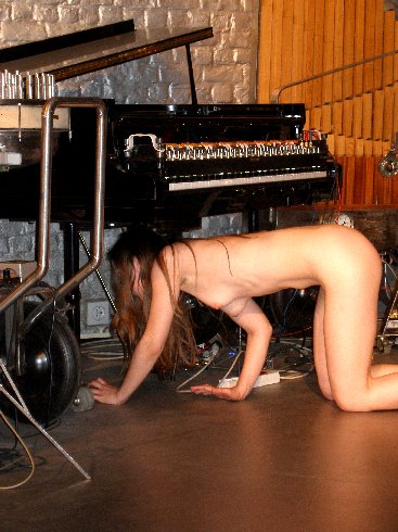
Their operating frequency is specified at 2.45GHz. The emitted electromagnetic waves are reflected by reflective surfaces and if in movement, these will cause a Doppler shift between emitted and reflected signal. As to human bodies, the most reflective surface is the naked skin. We performed measurements showing that a pullover gives a damping in the order of at least 12dB, thus reducing the resolution of the interface effectively with a factor 4 or worse. Hence our advise to always perform naked with this invisible instrument. Within the context of our own compositons, we make this nudity even compulsary.
Doppler formula:
fd = 2 v fo / c
so, after solving the device specific constants we get:
fd = 16.3 v
This holds for movements in line with the axis of the sensor. For other angles, the formula becomes:
fd = 16.3 v cos(a)
Where a is the angle between the movement and the axis of the sensor.
When we sample the signals at 128S/s, the highest detectable frequency would be 64Hz, conforming to the Nyquist theorem. So this limits the maximum detectable movement speed to
v = 64Hz / 16.3 or ca. 4m/s.
So if we want to be capable to resolve movement with higher speeds, we have to increase the sampling rate accordingly. Note however that moving human bodies never exceed speeds of 5m/s. Therefore sampling rates higher than 256S/s do not lead to any gain in information.
Signal amplitudes are inverse proportional to the square of the distance to the antenna and directly proportional to the size of the surface of the moving body. (6) The detection range for these devices is limited to 5 – 8 meters. Noise limits the range of the unit. Since we want the device to operate in real time, there is no way to resolve signals below or around the inherent noise level of the devices. The polar sensitivity, according the the Siemens datasheet, shows an opening angle of 120° (within -3dB):
Note that the device is not insensitive to movements to the sides and even to the backside, although the diagram does not show a lobe on the back. The devices each output two signals. The phase between them allows us to determine weather a body is approaching the antenna, or moving away from it. This phase angle can vary between 40° and 120° . Here again, for good phase angle resolution one should use the highest practical sampling rate.
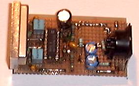
We designed a small circuit to perform some elementary signal conditioning on these output signals prior to presenting them to our A/D conversion device, thus relaxing the execution speed requirements for the data analysis software.
The first section is a 2-pole butterworth low pass filter with cut off at 64Hz and the second amplifier section serves as a 40dB gain preamp within the frequency band of interest. These parameters are optimized for use in combination with a 128S/s sampling rate. Note that, since we use 4 transducers each outputting 2 signals, we need a sampling device capable of sampling multichannels at a rate of larger than 1024S/s. In fact, the scanrate should be 128S/s and the time between samples for a single scan, as small as practical, since the more we approach real simultaneous sampling, the better our phase resolution will be. Use of a ICL7641 opamp in this circuit has the advantage that the output voltage can swing within millivolts to the power supply resp. ground terminals.(3) The DC level found on the Vd1 and Vd2 terminals of the sensor device, may vary from device to device (800mV to 1.3V), but seems to remain pretty stable over time and temperature. By adding a simple phase comparator circuit connected to both outputs, it is possible to derive an analog signal proportional to phase directly. Of course this can be handled in the software as well. A more sophisticated analog circuit using 5th order low pass filtering and the phase comparator will be published shortly on this page.
In our setup we use four circuits as described above. Since the bandwidth for each device is only ca. 100Hz, there is only a minimal chance that two of these circuits would happen to operate on a frequency less different than this bandwidth. In case this would be the case - Murphy being the way he is, this will happen on a crucial day or occasion- the setup will prove to be completely unworkable. You should select a different set of transducers, or play around a bit with the supply voltage, since operating frequency is to a certain extend a function of this parameter. (Do not go beyond the safe margins however: 10.8V to 15.6V for a frequency range of 2.4GHz to 2.48GHz). If you have equipment at hand, allowing precise measurement (within 0.01%) of frequencies into the GHz range, you should tune the radar modules such that they are at least 20kHz apart, thus avoiding all sorts of artifacts in the audio band.
The breadboard prototype of this sensor is shown on the picture below:
2. Adapter board to connect the outputs from these 4 devices to 8 A/D channels of a National Instruments PCMCIA data acquisition card (We use a DAQCard AI-16E-4, a 12bit 500kS/s device). This board also houses a linear stabilized power supply for the transducers. These require 12V dc and draw about 40mA each. This brings the total power requirements, including some safety margin to 12V/ 300mA, or no more than 4Watt. Standard 5pole 180° DIN connector cabling is used for the interconnections. A 68 pin (4 rows) male connector is provided to enable easy connection to the National Instruments PCMCIA DAQ card.
As we noted in earlier publications based on our research into microwave radar devices (1), the sensors used here can also be disturbed by ionising sources in their neighbourhood and range of sight. When using the 10 to 30GHz range, the effects of gasdischarge lights often made the use of the equipment problematic. With the sensors presented here, operating on the much lower frequency of 2.45GHz, this source of noise is strongly reduced but still exists. So the use of this equipment together with CRT's, TV-sets, TL-light, mercury vapor bulbs, our own digital loudspeakers, welding equipment, sodium vapor bulbs within a range of 10 meters around the setup should be discouraged.
Software
The software consists of two levels: a first level, a thread in its own, samples the signals from the transducers at the required sampling rate and processes this data such that we get access to following parameters:
To this end, a number of different algorithms are available for calculating this data set:
The inherent problem with the first two types of signal analysis -in this respect it is no different that what we stated with regards to ultrasonic technology in earlier reports- is that the signals do not typically show up really periodic components. The most relevant information is in the amount of deviation from periodicity. Acquiring this kind of information using FFT is generally speaking, not the best solution. Therefore we provided some alternatives as described above.
The musically most usefull results we got from using an algorithm counting the number of signal direction changes, larger than the noise level set, over the last second or less of data in the buffer. The default sampling rate, corresponding to the most useful setting after our experiments, is 128S/s. As to the derivation of most relevant information with regard to the amount of body surface moved, we found calculation of the root mean square of the most recent 500ms of the databuffer contents an optimum setting. We rescale the obtained value by taking its log2 value and multiplying it by 11.54. Thus we obtain a 'midi-compatible' 7-bit dynamic value directly.
The relevant procedures, including many more features than we can describe here, are integrated in our DLL library g_nih.dll. The source code is available. The required exported functions are:
GetRadarPointer (devicenumber) AS DWORD
this returns a pointer to the structure defined for each transducer. This structure behaves like an object and sets and returns all relevant data, operational mode and parameters. Devices are numbered 0 to 3.
The structure is defined in g_type.bi as:
TYPE RadarType DWORD alignment on dword boundaries pxbuf AS INTEGER PTR contains a pointer to the zero'th element of the databuffer (0 to 255) for the x-phase signal of a single sensor pybuf AS INTEGER PTR idem for the y-phase xa AS DWORD 11.54 times Log2 of the RMS amplitude, so the range is 0-127. The timewindow is 250ms. ya AS DWORD same for the y phase signal xal AS DWORD 11 bit amplitude value, over the last detected complete doppler period encountered in the x-phase signal yal AS DWORD idem, y-phase l AS SINGLE normalized distance based on the integrated rms signals from the x and y phase of a couple of transducers. Range 0-1 s AS SINGLE size of absolute surface of moving body as seen by the transducer v AS SINGLE absolute speed of slow (center of gravity) displacement of body acc AS SINGLE acceleration value of the above parameter pc AS COMPLEX cartesian coordinates of absolute position (0,0 = center of the setup) pl AS POLAR the same in polar coordinates xt AS SINGLE period of last x-phase doppler signal for internal use yt AS SINGLE period of last y-phase doppler signal for internal use xf AS SINGLE doppler frequency x-phase, not corrected with cosine of movement angle for internal use yf AS SINGLE idem. for y-phase for internal use vf AS SINGLE absolute value of fast movement speed based on the doppler shift frequencies received and with the cosine factor applied (in Hz) for conversion to physical units m/s you have to divide this value by 16.3. The range is 0.5 to 64Hz.(90Hz with cosine correction, but such values are unreliable) acf AS SINGLE absolute value of fast accelleration phase AS SINGLE phase angle between x and y phase signals for internal use noise AS LONG noise floor. Can be set by the user. can be set by the user dT AS DWORD Size of the time integration window, expressed in number of samples. Good values are between 16 and 80. The default is 64. can be set by the user params AS DWORD sets the algorithm for doppler frequency determination. Used with the declared constants: %ISOLWAVE, %DFT, %ZEROCROSS, %SIGNCHANGE, %ISOLPERIOD numeric values for these constants are in g_kons.bi setup AS DWORD sets the physical setup used for the radar transducers. Used with the declared constants:%SQUARE, %TETRAHEDRON, %FREE, %CUBE numeric values for these constants are in g_kons.bi END TYPE
In the software implementation we start by declaring an array of 5 variables of this type: r(0) to r(4), the last one just for holding global information on the detected movement from all transducers combined.
Radar_DAQ (param) AS LONG
this procedure starts / stops data acquisition from the connected transducers.
Declarations for these functions can be found in the file g_h.bi. Of course users do have to install the proper drivers for the DAQ card used (NiDAQ software from National Instruments). This software comes included with the purchase of any such device from National Instruments.
To derive musical meter and/or tempo information from the data acquired, one should apply a low pass filter with cutoff at 4Hz and store the buffered data in a memory array. A DFT performed on such a buffer with a data depth of 8 seconds will reveal gestural periodicity -if present- pretty well.
The derivation of meaningful information with regard to the gesture input is based on the same considerations and gesture typology as described in "Gesture controlled virtual musical instrument" (1999), with this difference, that the setup of the transducers in the form of a tetrahedron is not mandatory here. Of course, for the math involved to work well, one has to stick to the setup requirements and conditions implemented in the software.(4) The first set of studies developed so far, uses a diagonal cross setup (square) , since this makes determination of position in space pretty straightforward:
Let Ar1,Ar2,Ar3,Ar4 be the signal amplitude of the output of the sensors, fr1, fr2, fr3, fr4 the frequencies of the signals, S the surface of the moving body (for ease of calculation, we consider it is a sphere, seen as a circle by all sensors), k a scaling factor, L1, L2, L3, L4 the distances to the sensors. Then, in the setup as above we have:
Ar1 = k. S / (L1+1) ^ 2 and Ar3 = k.S/ (L3+1) ^ 2
as well as
Ar2 = k.S / (L2+1) ^ 2 and Ar4 - k.S / (L4+1) ^ 2
Thus we can write Ar1 / Ar3 = (L3+1)^2 / (L1+1)^2 as well as Ar2/ Ar4 = (L4+1)^2 / (L2+1)^2, so meaning that it is possible the locate the movement regardless the surface of the moving body parts. Of course the condition that there must be movement, holds. If we normalize the distance between opposite sensors (L1 + L3 = 1) , and state Q = SQR(Ar1 / Ar3) we simply get:
L1 = (2 - Q) / (Q + 1) and L3 = (2Q - 1) / (Q + 1)
Depending on the values of Ar1 and Ar3, it follows that the range for L1 and L3 becomes -1 to 2, meaning that we can also resolve positions beyond the space between both sensors. However, for our calculations we will limit the range to the traject 0-1. The size of the moving surface, as seen by the radar couple 1-3, can now also be derived as:
S1,3 = (Ar1.(L1+1)^2) = (Ar3.(L3+1)^2)
In practical measurement this equality will never be exact, but we can take advantage of this redundancy by increasing the certainty and calculating an average value for S as:
S1,3 = ((Ar1.(L1+1)^2) + (Ar3.(L3+1)^2)) / 2
The other pair of radars, 2-4, will similarly lead to the derivation of a value for S. Depending on the orientation of the moving body, this value will be different. The proportion between both values allows us to derive the orientation of the body within the square coordinates. Thus some information with regard to the shape of the moving body can be retrieved as well: the values of the size of the moving surface as seen by the radars 1 and 3 , and these seen by radars 2 and 4 will depend on the orientation of the moving body in the space: Since front and backside of a human body show more or less a twofold surface as compared to its sides, we can estimate the orientation or aspect of the moving body using this equation:
S1,3 / S2,4 = ((Ar1(L1+1)^2) + (Ar3(L3+1)^2)) / ((Ar2(L2+1)^2) + (Ar4(L4+1)^2))
Note that position determination as well as surface determination is also independent of movement velocity. This velocity however is also a function of the cosine of the movement angle. But, since we can calculate the position as shown above, it is now also possible to derive the absolute movement velocity. Moreover, we can do it with a lot of detail: in order to estimate the global velocity of the moving body, we can use the positional information against time: this works particularly well for very slow movements. For fast movements, we can use the available spectrum analysis with the cosine correction and retrieve information also about the spectral characteristics of the gesture waves (fluent, disruptive...).
Once we know L1, L2, L3 and L4, we can find the coordinates from the center of the setup (defined as point 0,0) as follows:
After conversion to polar coordinates, we get vector magnitude and angle. To derive the angle of movement we need to know two points on the traject of the movement:
ppc.real and ppc.imag for the previous point and pc.real = xpos and pc.imag = ypos the a more recent point. We now shift the line connecting these points (the movement traject) to the center of the coordinate system:
After conversion to polar, we now get p.mag and p.ang, and the cosine of p.ang is the factor by which we have to divide the frequency of the vector signal in order to get the absolute speed of the movement in the traject. At least, for the even (0 and 2) numbered transducers. For the odd ones (1 and 3) we can use the sine of the same angle. So:
This way the values returned in our structure , in the .vf field, are obtained. Since there is a fourfold redundancy, the found values can be averaged to reduce noise and inherent movement uncertainty. (5) If the signal amplitudes are high enough above the noise level, we can also derive relevant information with regard to the change of shape in time of the moving body. This can be very significant for dance movement analysis.
For a tetrahedral setup, the math involved is different and more complicated but pretty straigthforward as well. It has the advantage that we can derive full 3-dimensional positional information. Moreover, the uncertainty of the resulting values is much lower in this setup, since the angles all are one third smaller.
The data acquisition card we use has a 12 bit resolution. Since the normal noise level of the system is around 4, we should consider the last 2 bits as irrelevant. The practical resolution, and therefore the precision of the system, cannot be better than 10 bits. There is absolutely no advantage in using a higher resolution data acquisition card for this application. At least, unless lower noise or higher power microwave devices become available...
As a tool for evaluation, research and setup, we programmed a radar-display in GMT. The horizontal axis (line A-C) corresponds to the Radars 1 and 3, the vertical B-D, to 2 and 4. A blue ellipse is shown on the screen on the place where movement is detected. The size and aspect ratio of this ellipse is in proportion to the size and orientation of the moving body. The red polygon under or sticking out from the blue circle, gives an estimate of the certainty margins. Ideally, there should be no red visible for precize positional detection.
This radar screen is updated 16 times a second, so fast enough for a good video-like appearance.
Artistic applications
The <Quadrada> suite is a collection of studies in which we tried to explore different ways of mapping gesture information on musical activity produced by our robot orchestra, composed of following robots:
All the studies in this series, and
in fact all compositions by the author making use of any version of the invisible
instrument, have to be performed naked.
Study 1: "Slow et ruhig"
This was the first experimental study
we did perform in public using this equipment. The movements were performed
by specialized Butoh dancer Emilie De Vlam. The musical robots forming the M&M
ensemble, where the devices we mapped the gesture information on. This performance
took place at the Logos Tetrahedron, Ghent, 13th of February 2003. This study
uses only a single radar transducer.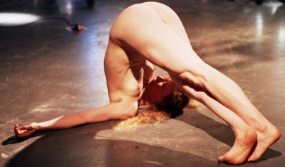
Study 2: "Birada"
This study uses two sensors, set up in line. The mapping makes use of <Piperola>, <Bourdonola>, <Harma>, <Vox Humanola>.
Study 3: "CatsPaws" [ Kattepoten]
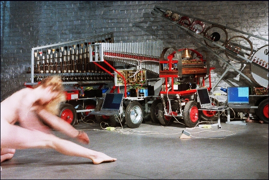
This uses the complete setup with all four sensors in a square configuration. It uses determination of spatial position to steer the pitches of our player piano in the piece. The tempo is mapped on non-positional movement speed. This piece was premiered in Enschede, on the M&M concert on friday march 7th, by Moniek Darge. In may 2009, we staged another version of this study with dancer and sound poet a.rawlings, combining vocal utterance with gesture.
Study 4: "Wandering Quadrada Space"
Using the complete square setup, this study maps positional information as well as acceleration and movement speed on the instruments of a robot orchestra composed of <Troms>, <Vox Humanola>, <Vibi>, <Harma>, <Piperola>, <Belly>, <Autosax>, <Bourdonola>, <Thunderwood> and <Springers>. Due to the high resolution required, nude performance is mandatory here. This piece was premiered by the author, on the M&M concert on thursday march 13th, 2003 in the Logos Tetrahedron in Ghent. After this premiere however, the piece was revized such as to become a lot more sensitive and demonstrative for the capabilities of this technology. The improved version was demonstrated on march 30th and 31th at the occasion of the "Technology Day" organised by the Flemish Government. It was performed again by the author on august 21 th of 2003, extended with the newly made robots <Tubi> and <So>.
This study was the point of departure for the act "Wandern" in our large scale music theatre composition "Technofaustus". In this new version, it was performed in The Hague on october 3th 2003 and at Vooruit in Ghent on octber 17th by Emilie De Vlam. On march 23th of 2004 it was performed again by the auhor.
Study 5: "Quadrada Vectorial"
This study uses an independent setup of four sensors. Absolute speed, surface and position information is not used here. We map de information from each sensor independently on the output of 4 to 8 of our robots: <Puff> on the A sensor, <Klung> and <Tubi> on the B sensor, <Player Piano> and <Vox Humanola> on the C sensor and <Vibi> and <Belly> on the D sensor.
This study was premiered on march 23th, 2004 by Emilie De Vlam, in the Logos Tetrahedron, Ghent. A new version was worked out with dancer/sound poet a.rawlings in 2009.
Study 6: "Qua Puff"
Demonstration piece using only a single transducer en mapping its output on the capabilities of our <Puff> automat. This piece was written for and performed by the author at the occasion of the Flemisch Technology day, march 14th 2004.
Study 7: "Qua Vibi"
Demonstration piece using only a single transducer en mapping its output on the capabilities of our <Vibi> and <Belly> automats.
Study 8: "QuAke"
This study uses <Ake> and <Harma>. It requires wide and slow movements.
Study 9: "Qua Llor"
This study uses <Llor> as well as <Belly>
Study 10: "Wet"
A study for our dripper automat.
Study 11: "Qua Vacca" (2005)
Premiered on tuesday november 8th, 2005 by Marian De Schryver.
Study 12: "Qua Vitello" (2006)
For the second cow-bell robot, after <La Vacca>
Study 13: "Qua Xy" (2007)
For the quartertone xylophone, <Xy>. Mapping on vector 1.
Study 14: "Qua Qt" (2007)
For the quartertone organ, <Qt>. Mapping on vectors 3 and 4. The studies for Puff, Qt and Xy can be played together. They use different vectors.
Study 15: "Qua Casta" (2007)
For the two robotic castenet players <Casta Uno> and <Casta Due>.Mapping
on vectors 1 and 2 for Casta Uno and 3 and 4 for Casta Due . The study can be
combined with "Wet". It may be performed with one or two butoh dancers".
Study 16: "Rotom" (2007)
This study uses a square or a tetrahedral setup, capable of fully using 3-dimensional space and gestural data. Sensors 0,1,2 are placed on the floor in an equilateral triangle and under an angle of 25° 15", sensor 3 is suspended over the center of the triangle. The distance between the sensors should be ca. 4 meters. It also works in a square setup. Each movement vector is mapped on a single rototom in the robot. Only the bass-drum responds to the overall gestural image. The piece is scored for one to four nude dancers.
Study 17: "Qua Simba" (2007)
In the works.
Study 18: "Tetrada"
This study uses a tetrahedral setup, capable of fully using 3-dimensional space and gestural data. Sensors 0,1,2 are placed on the floor in an equilateral triangle and under an angle of 25° 15", sensor 3 is suspended over the center of the triangle. The distance between the sensors should be ca. 4 meters.
The equipment is available for any competent composer wanting to develop a piece or performance using it. Since the use of the instruments requires software to be written, it is highly advisible to study our <GMT> software and its functionality with regard to this instrument. It is possible to use the equiment with other data acquisition systems, provided they can handle 8 channels, have 10 bit resolution and a reasonably fast sampling rate.
Other compositions by the author making extensive use of this equipment are "Transitrance", "Technofaustus" and "SQE-STO-4QR". In 2007 we used the same microwave devices in a hybrid gesture sensing device, wherein pulsed sonar is used for exact distance measurement and radar for gestural properties. A separate short paper on this project is available.
Dr. Godfried-Willem Raes
Notes:
(1) This project is part of the ongoing research of the author in gesture controlled devices over the last 30 years. Earlier systems, based on Sonar, Radar, infrared pyrodetection and other technologies are fully described in "Gesture controlled virtual musical instrument" (1999) as well as in his doctoral dissertation 'An Invisible Instrument' (1993). Artistic productions and compositions using these interfaces and devices have been: <Standing Waves>, <Holosound>, <A Book of Moves>, <Virtual Jews Harp>, <Songbook>, <Slow Sham Rising>, <Gestrobo>, <Technofaustus> etc.
(2) People interested in buying a system as described here can take contact with the author. Cost, depending on the version required, ranges from 4000€ to 10000 €, not including the required laptop computer. Delivery time is ca. 2 months.
(3) data with regard to these opamps are taken from: Intersil, Component Data Catalogue, 1986, p.4-34 to 4-49. Note that more commonly available opamps such as TLO74 will not work well in this application, for their very low frequency noise is excessive.
(4) A limitation of the square setup described here is that we basically retrieve all information in a plane. We have, unless a tetrahedral setup is used, no information with regard to possible vertical movement. Not that the square setup would be insensitive to vertical movement, since the sensitivity as follows from the polar diagram is hemispherical, but the information we retrieve is related to the projection of the movement on the plane connecting the four sensors. Future experiments will be performed using either a single suspended transducer or a cube using 8 transducers. Tetrahedral setups using 4 transducers, identical to the setup used for our sonar based invisible instruments, have been tested extensively as well.
(5) Complete source code for all math involved is available on the web at http://www.logosfoundation.org/gmt/gmt_dev/g_h.bas
(6) In some textbooks (Sinclair, 1992) on sensors we found the signal stated as being proportional to the square root of the surface... This is against our empirical findings.
Bibliographical references:
[Butoh dancer Emilie De Vlam in "Wandering Quadrada Space", 2004. The robots in the picture are (left to right), Klung, Tubi, Harma, Troms].
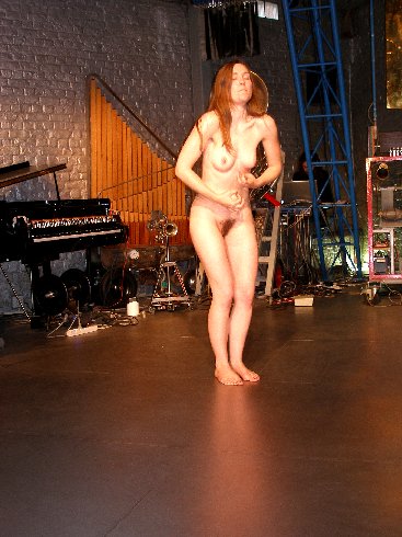
[Dancer and sound poet a.r. in Quadrada Study 'Catpaws', april 2009]
First published on the web: 15.01.2003 by dr.Godfried-Willem Raes
Last update:2017-03-23