<Namuda Gesture Recognition on the Holosound ii2010
platform>
by
dr.Godfried-Willem Raes
postdoctoral researcher
Ghent University, Ghent University College & Logos Foundation
![]()
2010
<Namuda Gesture Recognition on the Holosound ii2010
platform>
by
dr.Godfried-Willem Raes
postdoctoral researcher
Ghent University, Ghent University College & Logos Foundation
![]()
2010
This paper describes the software layer for gesture recognition
using doppler based hardware systems. For a good understanding it is advised
that readers familiarize first with the hardware described in "Holosound
2010, a doppler sonar based 3-D gesture measurement system ". This
paper is part of a triptych in which the last one will delve further into the
expressive meaning of gesture and on artistic aspects of the namuda dance project
developed at the Logos Foundation.
The holosound hardware is connected to the PC for sampling and further analysis,
treated in this preliminary draft of a paper. It is very important to stress
that all the data acquisition and classification procedures covered here were
designed to work concurrently and in real time. The latency was to be better
than 10ms. This restriction counts for the fact that we did not optimise the
procedures for maximalisation of precision nor for maximalisation of feature
extraction. It will be obvious that taking this restriction away, and performing
the analysis off-line, can greatly improve the functionality of the gesture
sensing technology for analytical and scientific purposes.
1. Data Acquisition:
Since the low pass filtering is performed in the hardware, we can set up a three-channel
sampler with a sampling rate of 1024 S/s. Using a National Instruments USB data
acquisition device (type: NI-USB 6210 or NI-USB 6212) and calling in the drivers
and libraries offered by NiDAQmx, this is pretty easy. The resolution is 16
bits and the voltage sensitivity for the inputs is programmed for -10 V to +10
V. Headroom is plenty such that we should not fear clipping. since the signals
from our hardware under normal circomstances stay well within the range of 4
Vpp. The data is read in a callback function operating at a rate of 256 times
a second. So on each call, 3 x 4 = 12 new samples are read. Reading the data
at the sampling rate itself is impossible due to limitations in the USB driver
implementation provided by National Instruments, this despite the fact that
the devices themselves can handle sampling rates well above 250 kS/s.
These samples are written to the fast circular data buffers, 256 entries in
size, one for each of the three vectors. Thus the time window available here
is 250 ms and the sampling rate remains at 1024S/s.
A medium size time window is setup in the same callback wherefore we downsample
to 256 S/s and write the result to the medium data buffers. Thus these circular
buffers cover a time window of 1 second, or, 256 samples. The downsampling applies
a simple low pass filter on the data.
A long time window, covering a 4 second timespan, is than implemented by downsampling
again to 64 S/s. These circular buffers again contain 256 samples.
Pointers to these nine circular buffers are made available to the user via a
specific structure. All buffer data is in double precision format and normalized,
bipolar -1 to +1.
Further preprocessing performed from within the same callback consists of:
A. setting up a running integrator with rectification in order to
calculate the signal strength proportional to the size of the moving and reflecting
body. These values are returned in the normalized .xa(), .ya(), .za() fields
of the structure. The integration depth can be controller with the parameter
in the .dta field.
The algorithm here also implements a high pass filter to eliminate slow DC offsets
and artifacts originated by very slow and mostly involuntary movements of the
body.
Summarizing, body surface derivation uses:
          high pass filter
          rectifier
          low pass filter
          integrator
B. Calculation of the frequencies in the doppler signals in order to grasp
information on the speed of movement. Here we encounter quite a few fundamental
problems: first of all, the signals are in no way periodic but in fact bandwidth
limited noise bands. Second, the frequency limits of these doppler signals depend
on the angle of the movement: the cosine in the doppler formula fd
= 2 v fo cos(a) / c. Only when movements are performed towards
or away from a particular vector in line with the transducer, the cosine will
be unity and the absolute value of the bandwidth trustworthy. If the performer
knows this, he/she can obviously take it into account. For general gesture analysis
though, ideally the coordinates of the movement in space have to be known. As
we proved in our papers and notes on hardware for gesture recognition, this
can be solved either by combining sonar and radar systems, or by FM modulating
the carrier wave. This adds a lot of complexity to the software and we will
not delve deeper into the related problems on this place.
However, even without cosine correction and lack of positional information,
we can reduce induced errors greatly by making use of the redundancy offered
by the fact that we have three vectors of data available. The sensors being
placed on the vertexes of an imaginary tetrahedron, make that the maximum value
for detected speed in the three vectors together can never be more than 50%
off, the cosine of 60 degrees being equal to 0.5.
The algorithm performed in the callback function, first converts the data in
the fast buffer to a square wave with a Schmitt trigger and hysteresis to avoid
noise interference. Then the zero crosses of the signal are counted, disregarding
any periodicity. Thus the results, returned in the .xf(), .yf(), .zf() fields
of our structure reflect noise densities of the signal, proportional to movement
speed. The numeric values returned are not normalized but reflect real world
values expressed in Hz, but to be interpreted carefully within the constraints
as laid out. If normalization is required, the values can be simply divided
by 200, a realistic maximum value as determined empirically.
C. Calculation of vectorial acceleration. This is done by differentiating the
vectorial frequency information. The delta-t value can be user controlled via
the .dtacc parameter. Larger values lead to better resolution at the detriment
of responsivenes. The results are returned in .xac(), .yac(), .zac() the scaling
being independent from the setting for .dtacc.
This callback function updates the parameter fields in the Doppler structure
256 times a second. This is the first level of processing of the movement data.
It yields information on the moving body surface as well as a first approximation
of speed.
Performing FFT's on the data buffers from within the same callback is impossible,
even on a quad core PC. Therefore the spectral analysis of the data must be
performed as a different thread. The shape of the spectrum (the distribution
of the frequency bands) reflects the characteristics of the gestures very well.
This can be demonstrated convincingly by mapping the output of the transform
on the keys of a piano, whereby the power of each frequency band is mapped on
the velocity of the attack for each key.
The complete structure as declared in the software is:
TYPE DopplerType DWORD      ' for ii_20xx with NiDAQmx
     xa     AS SINGLE       ' reflection amplitudes for the x-vector
     ya     AS SINGLE       ' idem for y-vector
     za     AS SINGLE       ' idem for z-vector
     xf     AS SINGLE       ' doppler frequency shift density for the x-vector
     yf     AS SINGLE
     zf     AS SINGLE
     xac    AS SINGLE       ' acceleration for the x-vector
     yac    AS SINGLE
     zac    AS SINGLE
     pxfast AS DOUBLE PTR   ' pointer to the x-vector data(0). Most recent data are in data(255) 250 ms buffer  1024 S/s
     pyfast AS DOUBLE PTR
     pzfast AS DOUBLE PTR
     pxm    AS DOUBLE PTR   ' 1s buffer, sampling rate 256 S/s
     pym    AS DOUBLE PTR
     pzm    AS DOUBLE PTR
     pxslow AS DOUBLE PTR   ' 4s buffer, sampling rate 64 S/s
     pyslow AS DOUBLE PTR
     pzslow AS DOUBLE PTR
     pxfbuf AS SINGLE PTR   ' 64 values for the frequency measurement, used for calculation of acceleration
     pyfbuf AS SINGLE PTR   ' sampling rate: 256 S/s
     pzfbuf AS SINGLE PTR   ' most recent data in data(63)
     dtacc  AS WORD         ' dt for acceleration derivation. Valid values: 1-63. Do not exceed range!
     dta    AS WORD         ' amplitude integration depth  (0-255)
     noise  AS SINGLE       ' noise level threshold   (1E-3, default, for 60 dB signal noise ratio)
     hpf    AS WORD         ' high pass filter differentiation depth
END TYPE
2. Gesture recognition
Although the callback function described above already performs quite some data
processing and allows us to get elementary information on the movement of the
body, it is not capable to perform gesture recognition. Hence the next steps.
In our approach, rather than trying to recognize predefined gesture models,
we attempt to maximalise the number of gestural characteristics retrievable
from the use of this particular hardware and its signals as used throughout
thousands of experiments with over 20 different human bodies. The subjects were
either trained musicians or dancers operating with direct auditory feedback.
We baptized these retrievable gestural characteristics as Namuda gesture prototypes.
Each prototype is defined within a certain timeframe (100 to 1000 ms) and has
a calculated normalized property strength as well as a persistence value, expressed
in time units (generally 1/256 second units, corresponding to the best possible
resolution within the constraints of our sampling function).
Namuda gesture types: (3)
Sofar we are able to distinguish twelve types (not counting the no-movement
property, 'Freeze'). We certainly do not exclude that it might be possible to
derive a few more, but at the other end we found that these twelve micro-gestures
might very well be already at the upper limit of what we can clearly control
given the motorics of our bodies. Many gestural characteristics can be seen
as dipoles: they exclude each other. Dipoles we distinguish are:
1.- Speeding up versus slowing down
speedup
definition: the movement speed goes up within a timeframe of maximum 500 ms
slowdown
definition: the movement speed goes down within a timeframe of maximum 500 ms
2.- Grow - Shrink ( or, expansion- implosion)
exploding
definition: the size of the moving body surface increases within a timeframe
of maximum 1000 ms
imploding
definition: the size of the moving body surface decreases within a timeframe
of maximum 1000 ms
Algorithms for feature extraction:
Speedup/slowdown and implode/explode use a gesture recognition algorithm based
on a FIR filter. The coefficients used are the elementary gesture type that
we are trying to evaluate. In the first approach these coefficients are linear
functions. Further refinement consists of applying different functions to calculate
the coefficients: quart sine or cosine, exponentials or even beta functions.
However, this should only be done on the condition that the pattern recognition
triggers the property with linear coefficients. The reason being that we simply
do not have enough computing power to handle each recognition algorithm with
many different coefficient models in real time.
The procedure is implemented as a function to which the pointer to the frequency
data array (covering 500 ms) is passed as well as the vector. Vectors are numbered
0,1,2 for the x, y, and z vertexes where the transducers are placed physically.
Vector 3 always refers to a sum or a maximum value. (2)
SUB GestureProp_Speedup (BYREF ar() AS SINGLE, BYVAL vektor AS LONG)
    'time weighted moving average approach using a Nth order FIR filter
    'vector: 0,1,2  for x,y,z
    'speed data   - the coefficients are the shape of a speedup gesture (rising)

    LOCAL i AS DWORD
    LOCAL av AS SINGLE
    STATIC order AS LONG
    STATIC Fscale  AS SINGLE
    DIM oldF(0 TO 2) AS STATIC SINGLE

    ' speedup coefficients, these have only to be recalculated if the window size is changed with .Forder:
    IF order <> gesture.Forder THEN
        order = gesture.Forder
        REDIM bs(0 TO order) AS STATIC SINGLE
        RESET Fscale
        FOR i = 0 TO order
            bs(i) = i / order                 'rising series of coefficients: this is the gesture model
        NEXT i
        Fscale = (order + 1) / 2              'for normalization
    END IF

    'FIR with time dependent linear coefficients:
    FOR i = (UBOUND(ar) - order) TO UBOUND(ar)
            av = av + (ar(i) * bs(i-UBOUND(ar) + order))
    NEXT i

    'now we calculate the matching value (fuzzy):
    IF av > oldF(vektor) THEN
          gesture.speedup(vektor) = (av - oldF(vektor)) * 2
          INCR gesture.speedup_dur(vektor)
    ELSE
          RESET gesture.speedup(vektor), gesture.speedup_dur(vektor)
    END IF
    gesture.speedup_val(vektor) = av/ Fscale 'this is the renormalised output value of the filter itself
    oldF(vektor) = av

    'reconsider the global property (vektor 3):
    Gesture.speedup(3) =  MAX(Gesture.speedup(0), Gesture.speedup(1),Gesture.speedup(2))
    Gesture.speedup_val(3) =  MAX(Gesture.speedup_val(0), Gesture.speedup_val(1),Gesture.speedup_val(2))

END SUB
Here is a plot of the result of this algorithm:
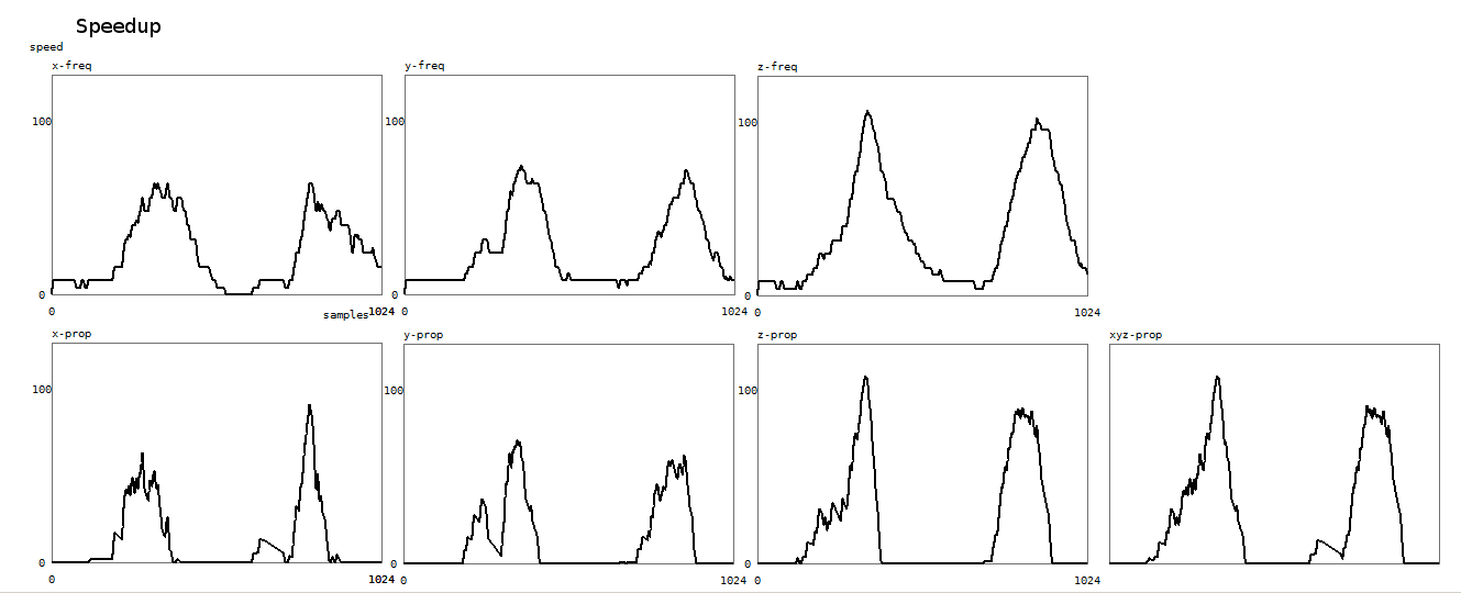
The upper three graphs give the frequency signals for the x,y and z vectors
as found in pDoppler.xf, yf, zf. Vertical scale is in Hz. The window shows a
timeframe of 4 seconds. The graphs below show the output of the recognition.
The vertical scale shows property strength, again for the three vectors. The
last graph shows the property for all three vectors together.
The procedure for slowdown recognition is identical, but the coefficients are
a linearly descending series.
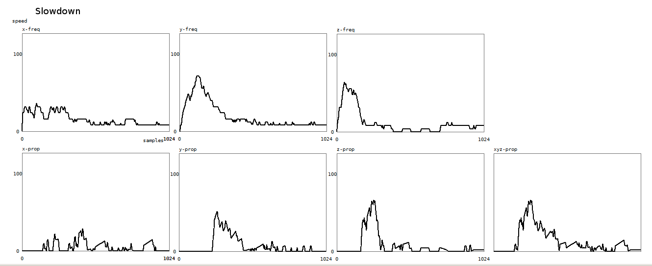
Here is a plot of the result of the slowdown recognition algorithm:
For shrinking/expanding body surface we use the same approach but found that
the time window has to be taken larger for a good reliability. We have it set
at 1 second. The FIR filter order can be changed by the user using the parameter
in the .Sorder field.
Here is the procedure for shrinking gesture recognition with linear coefficients:
SUB Gestureprop_Shrink ((BYREF ar() AS SINGLE, BYVAL vektor AS LONG)
    ' pattern recognition code using FIR approach with the gesture model based in the coefficients
    ' since this works with our omnidirectional ii2010 receivers , no angle correction is required
    ' the amplitudes of the reflected signals are independent from the frequency of the doppler shift.

    LOCAL i,j AS DWORD
    LOCAL av, s AS SINGLE
    STATIC order AS LONG
    STATIC Sscale  AS SINGLE
    DIM oldS(0 TO 2) AS STATIC SINGLE
    DIM bs(0 TO gesture.Sorder) AS STATIC SINGLE

    'calculation of a descending series of coefficients:
    IF order <> gesture.Sorder THEN
        order = gesture.Sorder
        REDIM bs(0 TO order) AS STATIC SINGLE
        RESET Sscale
        FOR i = 0 TO order
            bs(i) = 1 - (i/(order+1))               'this could also be the result of a beta-function describing the gesture type
            Sscale = Sscale + bs(i)                 'sum of factors, required for normalisation.
        NEXT i
    END IF

    'FIR filter with time dependent linearly descending coefficients:
    RESET j
    FOR i = (UBOUND(ar) - order + 1) TO UBOUND(ar)
            av = av + (ar(i) * bs(j))
            INCR j
    NEXT i

    'now classify: shrinking surface
     IF (av < oldS(vektor)- (@pDoppler.noise/ SQR(order)))  AND (av/Sscale > @pDoppler.noise) THEN
          IF gesture.implo_dur(vektor) THEN
                   gesture.implo(vektor) = MAX(MIN((oldS(vektor) - Av)* 2.5, 1),0)
                                                          'scaling factor for commensurability with the explo property
                                                          'observed range, before rescaling with * 2.5:
                                                          '19.04: x<= 0.156, y<=0.224, z<=0.08  [gwr with clothes]
                                                          '19.04: X<= 0.335, y<=0.373, z<=0.268 [gwr naked]
          ELSE
                  RESET gesture.implo(vektor)
                                                          'the property will only be set if it lasts at least 7.8ms
          END IF
          INCR gesture.implo_dur(vektor)                  'in 1/256s units (3.9ms).
     ELSE
                  RESET gesture.implo(vektor), gesture.implo_dur(vektor)
     END IF
     gesture.implo_val(vektor) = av/ Sscale   'we always return this normalized value for research purposes.
     oldS(vektor) = av

    gesture.implo(3) =  (gesture.implo(0) * gesture.implo(1) * gesture.implo(2)) ^0.33   'to be further investigated
    gesture.implo_val(3) =  (gesture.implo_val(0) * gesture.implo_val(1) * gesture.implo_val(2)) ^0.33

END SUB
Here is a plot of the result of the implosion algorithm:
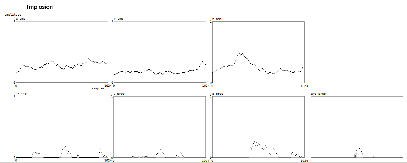
In this case we plot in the upper three graphs the normalised amplitudes of the doppler signals against time (4 seconds). Below, again property strength.
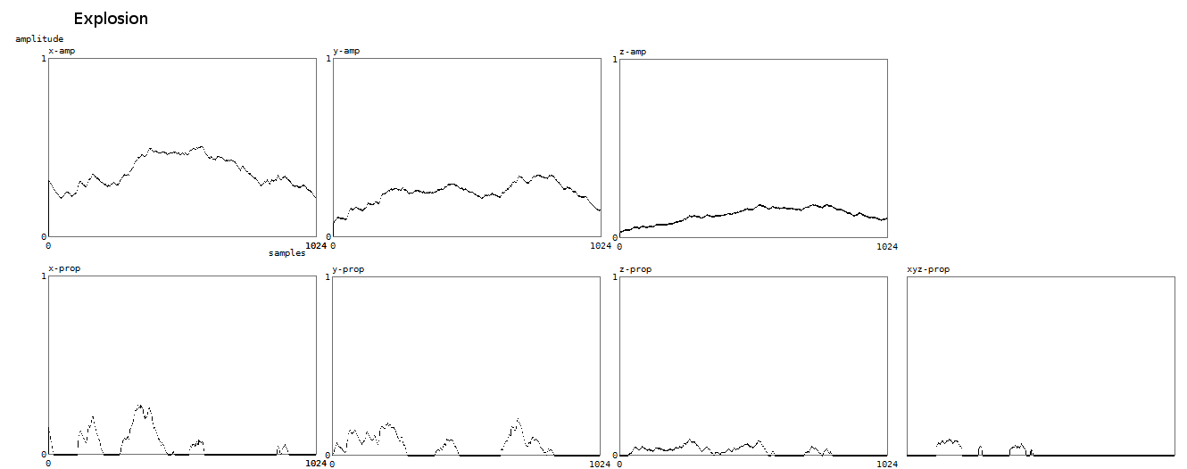
For explosion we get similarly:
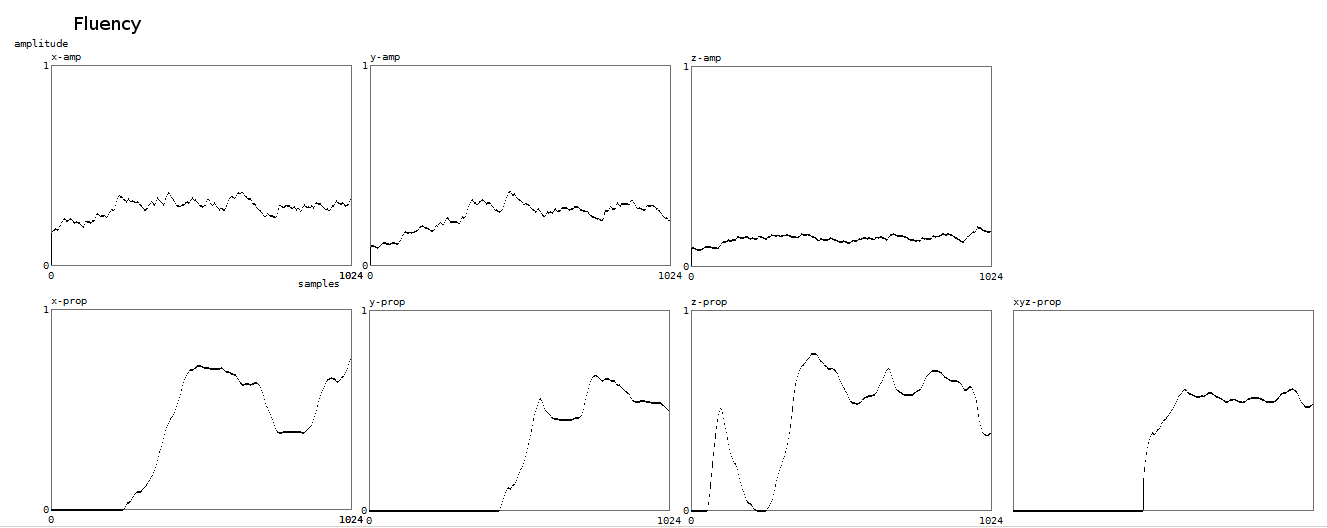
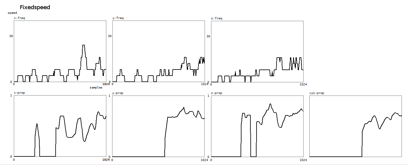
3. Fluency and speed properties
Not all gesture properties are calculated with this or a similar FIR algorithm.
For the properties fluency (constancy of moving body surface within the timeframe)
and fixspeed (constancy of movement speed within the timeframe), we found traditional
statistics useful. Here we look in the databuffer and calculate the running
average as well as the significance. The smaller the deviation from the mean,
the stronger the property will be evaluated.
Here is, as an example, our coding for fluency detection:
SUB Gestureprop_Fluent ((BYREF ar() AS SINGLE, BYVAL vektor AS LONG)
    LOCAL avg, d, s AS SINGLE
    LOCAL i AS DWORD
    STATIC maxval, maxprop AS SINGLE

         ' calculation of the average in the body surface data array:
        FOR i = 0 TO UBOUND(ar)
            Avg = Avg + ar(i)
        NEXT i
        Avg = Avg / (UBOUND(ar) +1)        'normalised 0-1

        'calculate the standard deviation:
        FOR i = 0 TO UBOUND(ar)
            d = d + ((ar(i) - Avg)^ 2)     ' method of the smallest squares
        NEXT i                             ' d =  average fault for each sample
        s = SQR(d/(UBOUND(ar)-1))          ' s = standard deviation for a random population

            ' statistics math memo:
            ' 68% of all values in dta are between Avg - s and Avg + s
            ' 95%                      are between Avg -2s and Avg +2s
            ' 97%                      are between Avg -3s and Avg +3s

            IF Avg > @pDoppler.noise * 5  THEN
                IF gesture.flue_dur(vektor) THEN
                    gesture.flue(vektor) = MAX(0, 1 - (5*s / Avg))   'gives quite a good range
                ELSE
                    RESET gesture.flue(vektor)
                END IF
                INCR gesture.flue_dur(vektor)
            ELSE
                RESET gesture.flue(vektor), gesture.flue_dur(vektor)
            END IF
            gesture.flue_val(vektor) = Avg                            ' always returned.

        Gesture.flue_val(3) = (Gesture.flue_val(0) * Gesture.flue_val(1) * Gesture.flue_val(2)) ^ 0.33  ' questionable
        gesture.flue(3) = (gesture.flue(0) * gesture.flue(1) * gesture.flue(2)) ^ 0.33

END SUB
Here is a plot of the result of the fluency property algorithm:
 `
`
And here, again for the speed constancy property:
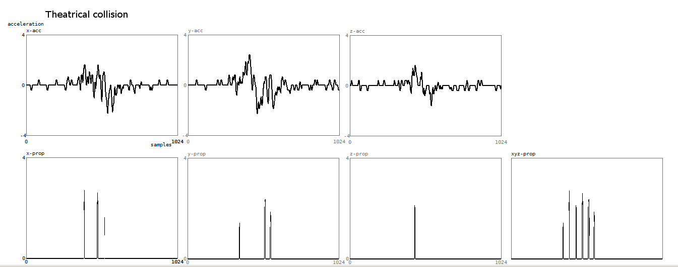
4. Collision - Theatrical Collision
For the dipole collision/theatrical collision, we use yet another approach,
based on an analysis of the acceleration data acquired in the sampling callback.
The time window used in this analysis is 100 to 390 ms. The smaller values make
the algorithm more responsive.
We define the collision property as follows:
the acceleration rises up to the point of collision, where we have a sudden
sign reversal.
And, the theatrical collision as:
the acceleration goes down to the point of collision -a standstill- , where
we have a small sign reversal followed with a rise of acceleration.
Algorithm:
a first leaky integrator is applied on the first 3/4th's of the acceleration
data (upval) and a second integrator on the last quart of the data (downval).
The sensitivity is set with the variable sens.
If now upval > sens and downval < - sens, we set the collision property.
The practical coding is as follows:
SUB Gestureprop_Collision (BYREF ar() AS SINGLE,  BYVAL vektor AS LONG)
    ' the array passed should be the amplitude array, we need it to look up the impact value on the moment of the collision
    ' we could also pass the value ar(230) alone.
    ' the algo uses a leaky integrator, not FIR!, on the acceleration data
    ' the procedure returns the gesture properties collision and theatrical collision. These are mutually exclusive.
    STATIC tog AS LONG
    STATIC xslope, yslope, zslope, xdown, ydown, zdown, sens AS SINGLE
    IF ISFALSE tog THEN
            sens = 0.4                             ' this is a critical value to experiment with
            DIM xc(0 TO 25) AS STATIC SINGLE       ' 101 ms buffers for acceleration and collision
            DIM yc(0 TO 25) AS STATIC SINGLE       ' empirically determined
            DIM zc(0 TO 25) AS STATIC SINGLE
            tog = %True
    END IF

    SELECT CASE vektor
           CASE 0
                   ARRAY DELETE xc(), @pDoppler.xac    ' circular buffer with acceleration data. Most recent data now in xc(last)
                   'calculate the shape:
                   xslope = (xslope + xc(0)) / 2       ' low pass filter - should cut off around 25Hz
                   xdown = (xdown + xc(25)) /2
                   IF (xslope > sens) AND (xdown < -sens) THEN       ' this is the pattern recognition condition
                            Gesture.collision(0) = xslope - xdown    ' always positive, since xdown is negative !
                            INCR Gesture.collision_dur(0)
                            Gesture.impact(0) =  ar(230)             ' further research required for optimum value in the array
                            RESET Gesture.theacol(0), Gesture.theacol_dur(0)
                   ELSEIF (xslope < -sens) AND (xdown > sens) THEN    ' condition for theatrical collision
                            Gesture.theacol(0) = xdown - xslope       ' always positive, since xslope is negative !
                            INCR Gesture.theacol_dur(0)
                            RESET Gesture.collision(0),  Gesture.collision_dur(0)
                            Gesture.impact(0) =  ar(230)
                   ELSE
                            RESET Gesture.collision(0), Gesture.theacol(0), Gesture.impact(0)
                            RESET Gesture.collision_dur(0), Gesture.theacol_dur(0)
                   END IF
           CASE 1
                   ARRAY DELETE yc(), @pDoppler.yac    ' the accelleration values are updated 256 times a second
                   yslope = (yslope + yc(0)) / 2
                   ydown = (ydown + yc(25)) / 2
                   IF (yslope > sens) AND (ydown < -sens) THEN
                         Gesture.collision(1) = yslope - ydown
                         INCR Gesture.collision_dur(1)
                         Gesture.impact(1) = ar(230)
                         RESET Gesture.theacol(1), Gesture.theacol_dur(1)
                   ELSEIF (yslope < -sens) AND (ydown > sens) THEN
                         Gesture.theacol(1) = ydown - yslope
                         Gesture.impact(1) =  ar(230)
                         INCR Gesture.theacol_dur(1)
                         RESET Gesture.collision(1),  Gesture.collision_dur(1)
                   ELSE
                         RESET Gesture.collision(1), Gesture.theacol(1), Gesture.impact(1)
                         RESET Gesture.collision_dur(1), Gesture.theacol_dur(1)
                   END IF
           CASE 2
                   ARRAY DELETE zc(), @pDoppler.zac
                   zslope = (zslope + zc(0)) / 2
                   zdown = (zdown + zc(25)) / 2
                   IF (zslope > sens) AND (zdown < -sens) THEN
                        Gesture.collision(2) = zslope - zdown
                        Gesture.impact(2) = ar(230)
                        INCR Gesture.collision_dur(2)
                        RESET Gesture.theacol(2), Gesture.theacol_dur(2)
                   ELSEIF (zslope < -sens) AND (zdown > sens) THEN
                        Gesture.theacol(2) = zdown - zslope
                        Gesture.impact(2) =  ar(230)
                        INCR Gesture.theacol_dur(1)
                        RESET Gesture.collision(2),  Gesture.collision_dur(2)
                   ELSE
                        RESET Gesture.collision(2), Gesture.theacol(2), Gesture.impact(2)
                        RESET Gesture.collision_dur(2), Gesture.theacol_dur(2)
                  END IF
    END SELECT

    Gesture.collision(3) = MAX(Gesture.collision(0), Gesture.collision(1), Gesture.collision(2))
    Gesture.theacol(3) = MAX(Gesture.theacol(0), Gesture.theacol(1), Gesture.theacol(2))
    IF Gesture.collision(3) THEN
        Gesture.impact(3) = MAX(Gesture.impact(0), Gesture.impact(1), Gesture.impact(2))
    ELSEIF Gesture.theacol(3) THEN
        Gesture.impact(3) = MAX(Gesture.impact(0), Gesture.impact(1), Gesture.impact(2))
    ELSE
        RESET Gesture.impact(3)
    END IF

END SUB
Here is a plot of the result of the collision detection algorithm:
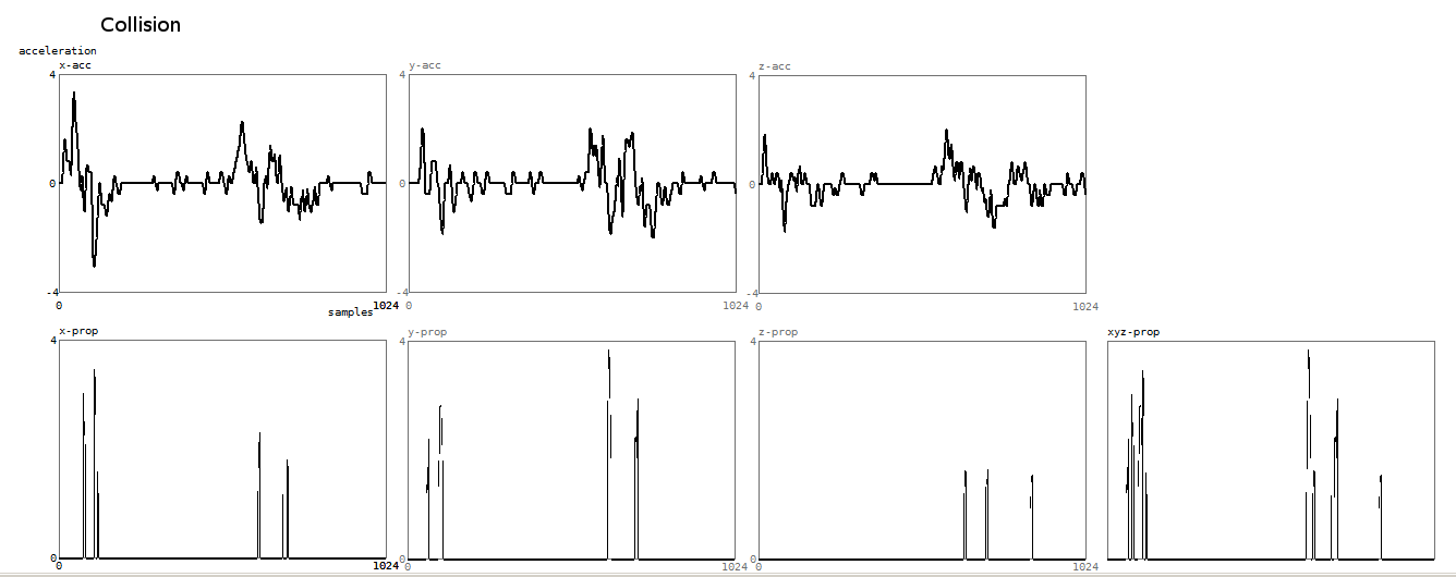
In this case the upper graphs show the vectorial accelleration channels. Theatrical collision detection resulted in the graphs below:
5. Roundness - Edginess
The spectral analysis of the doppler signals in the short data buffer allow
us to discriminate gesture properties situated on a dipole that can be described
as 'roundness' versus edginess. Other ways to describe the gesture characteristic
referred to could be smooth and shaky or jagged.
definition: roundness applies if the gestures are smooth and continuous; edginess,
if the gestures contain many abrupt components and discontinuities. The property
reflects aspects of the shape of a gesture very well.
The analysis is based on the spectral power distribution in the fast data buffer
(250ms). The code as we wrote it at first for the fourier transforms is:
SUB DFT_Dbl (Samp#(), Sp#()) EXPORT
'discrete fourier transform on double precision data
LOCAL x, i, maat, halfsize AS LONG
LOCAL kfaktor#, kt#, Rl#, Im#, g#, pw#
DIM a(UBOUND(Samp#)) AS LOCAL DOUBLE
maat = (UBOUND(Samp#)) + 1 ' must be a power of 2
halfsize = maat / 2
'note: size of Sp# must be Sp#(halfsize-1)
kfaktor# = Pi2 / maat ' this is eqv. to ATN(1)* 8# / maat
MAT a() = (1.0/maat) * Samp#()
i = 0
DOkt# = kfaktor# * iLOOP UNTIL i = halfsize ' the second half would be empty
RESET Rl# , Im#
FOR x = 0 TO maat - 1
g# = (kt# * x)NEXT x
Rl# = Rl# + (a(x) * COS(g#))
Im# = Im# - (a(x) * SIN(g#))
pw# = (Rl# * Rl#) + (Im# * Im#) ' sum of squares
IF pw# THEN Sp#(i) = 2 * SQR(pw#)
INCR i
END SUB
In a later 10-fold improvement for speed, we recoded this using lookup tables for the sine and cosine factors and added the application of a hanning window inline. The resulting code becomes obviously a lort less readible. All DFT's in our gesture recognition code are performed with a 25% overlap. To classify these properties, we split the power spectrum frequency bins in Sp#() in two parts at a variable point i. Note that our spectrum is 8 octaves wide (4 Hz to 512 Hz) and thus, taking into account the linear nature of the frequency distrtibution in the transform, we have to set i=15 for a normal midpoint at 64Hz. Then we sum up the power in the spectral bands up to i, as well as the power in the spectral bands i+1 up to the highest frequency. The power found in the lowest bin at Sp#((0) is dropped. If lw is the first sum, and hw the second, the smoothness property for each vector is calculated as 1 - (lh / (lw+lh)) and for the edgy property as 1 - (lw/(lw+lh)). The structure returns also the durations of these mutually exclusive properties in 1/256 s units. The algorithm for this property runs at a much lower speed of 16Hz, thus guaranteeing a data overlap of 25% on each refresh. Performing the required transforms much faster, causes to much jitter in the behaviour of our real time multitasker. A consequence of this is that the durations are incremented in 16 unit steps (62.5 ms).
As we found that the analysis of the power spectrum offers a good base for the analysis of some gestural features, we created a thread in the software to perform the spectral transforms on all three databuffers continuously. The results are returned to the user via pointers in the gesture structure: gesture.pspf() for the fast transform (4 Hz-512 Hz in 128 bands, with a refresh frequency of 25 Hz); gesture.pspm() for the medium buffer transform (1 Hz- 128 Hz in 128 bands, with a refresh frequency of 5 Hz), gesture.psps() for the slow buffer transform (0.25 Hz- 32 Hz in 128 band, with a refresh frequency of 1.25 Hz).
6. Airborness
We came upon this gesture property, when doing experiments with balls thrown through the sensor system. When looking into the spectral analysis data obtained, we noticed that for flying objects, the spectrum is discontinuous and reveals a gap on its low end. By looking at the size of the gap, we can distinguish flying objects -or for that matter, similarly, acrobatic jumps- from bodies in contacts with the ground. The reason for this is quite easy to understand, if we realize that a moving body normally always has some parts at rest, even when extremities such as arms, legs, head are moving vehemently. The doppler noise bands returned are therefore continuous and start always at zero. Airborness might not be the most usefull feature to extract from musicians gesture, but forms an attractive bonus if it comes to dance movement analysis. It will be obvious that the timeframe for this property detection has to be taken very short and that the persistence values of the property cannot attain high values.
When coding for recognition of this property, one has to be very carefull to take into account the spread of the background noise in the spectrum. To clarify this, we give here a plot of the maxima encountered in the spectral transform over the 250ms time window (x-vector) without any body in the setup:
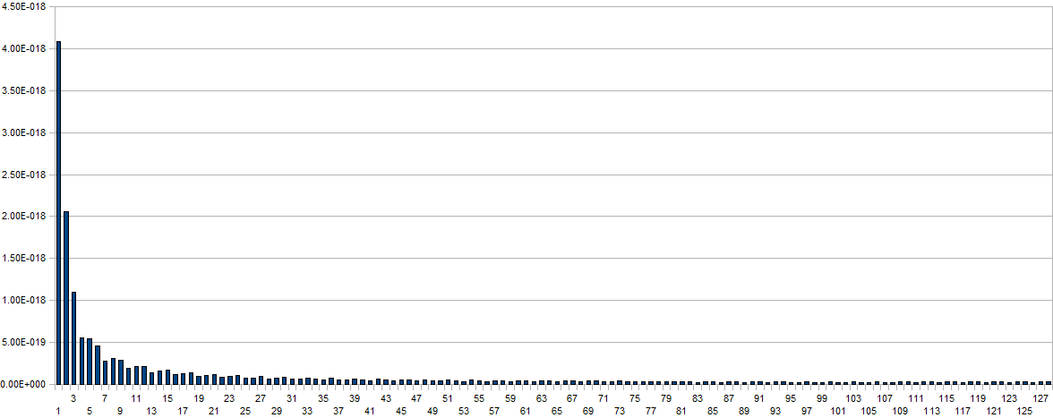
The values on the horizontal axis are the frequency bins and have to be multiplied with a factor four to obtain real world frequency values. Measurement time for this plot was 2 minutes. For proper evaluation of spectrum based gesture properties, this basic noise spectrum has to be subtracted from the acquired data arrays. From a scientific point of view the superiour way of handling this would be by letting the software measure the basic noise spectrum on initialisation. Taking into account the stringent conditions for a meaningfull measurement (no moving bodies nor objects in the neighourbood as well as a measurement time of a few minutes), we rather used a rough approximation of the curve in our coding. Here are two typical spectrum plots thus obtained during a jump:
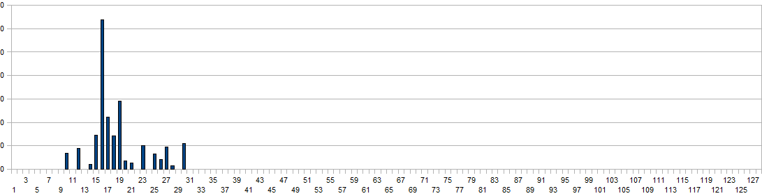
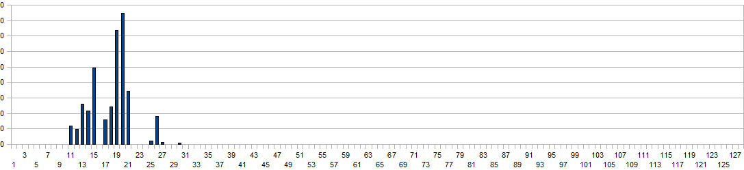
The vertical scaling was adapted a factor 10, to cope with the higher dynamic range obtained here. Unfortunately, due to the refresh speed limitations of the transforms in our coding, this property can only be calculated at a rate of 8 times a second. Hence, the duration field returns only a rough estimate of the time the body is airborne and cannot be used for precise measurement of jumps. However, the shape of the gesture during the jump is pretty well reflected in the obtained spectrum. In order to optimize the recognition code for speed, we convert the spectra to octave-bands first. Then we evaluate the proportion of power distribution in the lowest two bands to the sum of all the higher bands. If the total power is higher than a measured noise level and this proportion exceeds an empirically determined value (a value of 17 was found), the property is set. The reliability of jump detection using this algorithm is higher than 90%.
7. Tempo and periodicity
The most difficult gesture property to retrieve in real time is periodicity.
It represents a well known problem that has been treated in depth by a lot of
different authors in very different contexts. The problem is the same, whether
applied to music or to gesture. We need information about periodicity in the
gesture because it allows us the derive a tempo from gesture input.
There are a number of different algorithms possible, each with pro and cons.
Since we are dealing with slow periodic phenomena, the fastest algorithm consists
of measuring the time between periods (1/t equals frequency then) and checking
the deviation from the mean on each new periodic phenomenon. The fastest algorithm
starts from the collision detector, and yields a delay time in the order of
100ms. Synchronization is well possible, but latency and sudden jumps cannot
be avoided. For clearly colliding periodic gestures, this method is very reliable
and precise as long as the periodicity stays below 4 Hz (tempo MM240). However
it imposes many restrictions on the type of gesture input. The jitter on the
periodicity can be used as a base to calculate a fuzzy value for the tempo property.
For conducting kind of gestures we found that this path can be followed although
the results are not always very convincing.
The FFT approach can be followed as well, but since it has to work on the 4
second buffers if it is to resolve tempi as low as MM30, the latency will be
very large. The advantage is that it also works on less clear-cut gesture input.
A serious disadvantage is that synchronizing with the input is difficult. The
code as we wrote it, tries to cancel out the frequent occurrences of harmonics
in the spectral transforms. Yet, it is far from perfect although we have been
using it to synchronize music coded in midi files or calculated in real time
with dancers on stage.
In the FFT approach, we coded a task that tries to derive a musical tempo expressed in MM numbers by interpollating between the frequency bins from the spectrum transforms. Here is a code snippet:
' spectra obtained after a DFT with a hanning window in the FFT thread
' vectors are 0,1,2 for the x,y,z buffers and 3 for the sum.
DIM sps(128) AS LOCAL DOUBLE AT @gesture.psps(vector)
i = ArrayMax_Dbl (sps()) 'find the strongest frequency bin
IF i THENgesture.periodic(3) = ((i+1) * 15) - (7.5 * sps(i-1)/sps(i)) + (7.5 * sps(i+1)/sps(i))ELSE
gesture.jitter(3) = (SQR(sps(i) + sps(i-1) + sps(i+1))) * 1E9gesture.periodic(3) = 15 + (7.5 * sps(1)/sps(0))END IF
gesture.jitter(3) = (SQR(sps(0) + sps(1))) * 1E9
' now we try to evaluate the spectrum
RESET ct
FOR i = 0 TO 2IF ABS(gesture.periodic(i) - gesture.periodic(3)) < gesture.periodic(3)/ 20 THEN ' 5% deviation allowedNEXT iINCR ctELSEIF ABS((gesture.periodic(i)/2) - gesture.periodic(3)) < gesture.periodic(3)/ 20 THENINCR ct 'in this case the i vector must be an octave above the sum of vectorsELSEIF ABS((gesture.periodic(i)*2) - gesture.periodic(3)) < gesture.periodic(3)/ 20 THENINCR ct 'in this case the i vector must be an octave below the sum of vectorsELSEIF ABS((gesture.periodic(i)/3) - gesture.periodic(3)) < gesture.periodic(3)/ 20 THENINCR ct 'in this case the i vector must be an fifth above the sum of vectorsEND IF
SELECT CASE ctCASE 0END SELECT
gesture.jitter(3) = gesture.jitter(3) ^4 ' no periodicityCASE 3 ' here we are certain, although we may have the wrong octave.
gesture.jitter(3) = gesture.jitter(3) ^ 0.25CASE 2 ' high probabilitygesture.jitter(3) = gesture.jitter(3) ^ 0.5 ' we should see how the one deviating period relates to the equal ones.CASE 1
' if it is a harmonic, we could increase confidencegesture.jitter(3) = gesture.jitter(2) ^ 1.5 ' decrease certainty
Suggestions for improved code here are most welcomed.
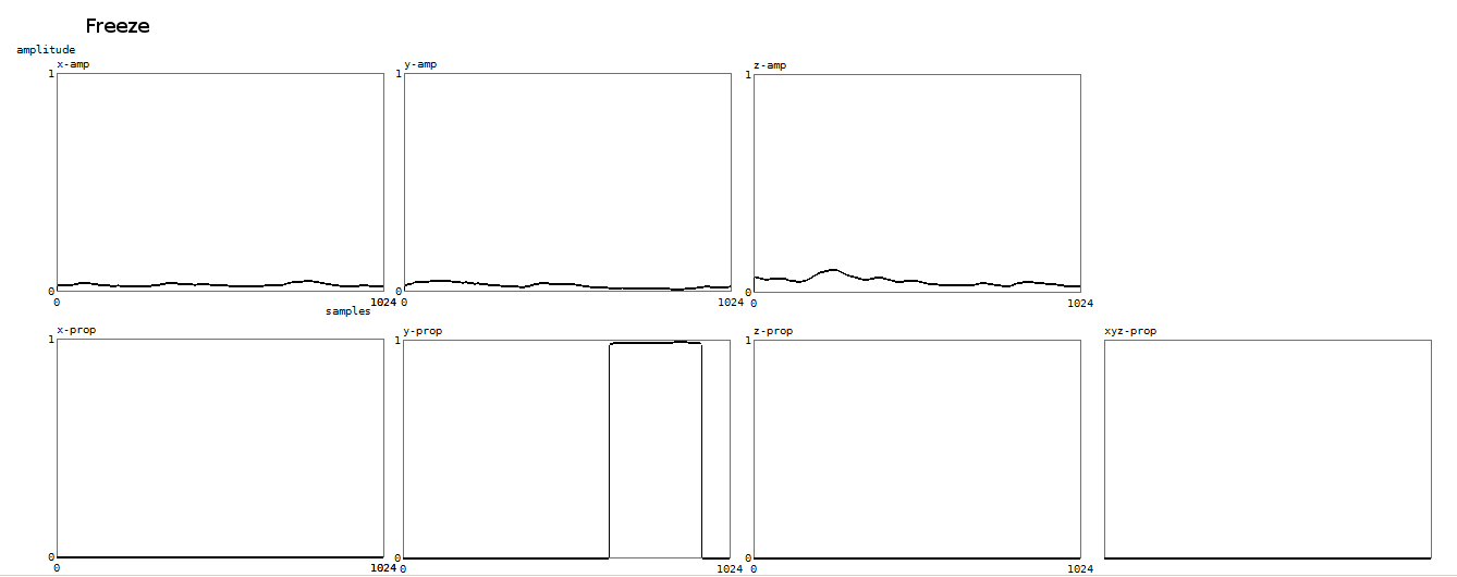
8. Freeze
A gesture property almost so trivial that we would almost forget to mention
it: the absence of movement. We could also have named it rest, referring to
the musical meaning. Absence of movement can be detected as soon as the received
signals are sinking away in the noise floor. This happens when no body is in
the setup. A gesture freeze with a body in the field of the sensors will always
have signal levels above absolute noise, since a living body always moves. Therefore,
this property is not binary, but again a fuzzy value with a duration of its
own.
Here is a plot for the freeze property, wherein only for the y-vector the property gets set:
As of the time of the writing, the structure used to return our gesture properties to the user looks like:
TYPE GestureType DWORD
     collision (3) AS SINGLE         '0=X, 1=Y, 2=Z, 3= total     acceleration based, the values are the correlation magnitude
     collision_dur (3) AS LONG       'in 1/256 s units
     theacol   (3) AS SINGLE         'theatrical collision        acceleration based
     theacol_dur (3) AS LONG         'in 1/256 s units
     implo     (3) AS SINGLE         'surface based  - normalized property strength
     implo_dur (3) AS LONG           'in 1/256 s units 0 at the start of detection, climbing up as long as the property is valid.
     implo_val (3) AS SINGLE
     explo     (3) AS SINGLE         'surface based  - normalized property strength
     explo_dur (3) AS LONG           'duration of the property in 1/256 s units
     explo_val (3) AS SINGLE         'prediction value of the property (FIR output)
     speedup   (3) AS SINGLE         'speed based
     speedup_dur (3) AS LONG
     speedup_val (3) AS SINGLE
     slowdown  (3) AS SINGLE         'speed based
     slowdown_dur (3) AS LONG
     slowdown_val (3) AS SINGLE
     periodic  (3) AS SINGLE      'should give the tempo in MM units
     jitter    (3) AS SINGLE      'should give the degree of certainty of the above tempo.
     flue      (3) AS SINGLE      'gives the standard deviation for the surface buffer  (in fact 1-s)   constant body surface property
     flue_val  (3) AS SINGLE      'gives the average value for the surface buffer   (normalized 0-1)    size of body surface
     flue_dur  (3) AS LONG        'duration in 1/256 s units
     fixspeed  (3) AS SINGLE      'speed based, gives standard deviation for the frequency buffer
     fixspeed_val (3) AS SINGLE   'gives the average value of the constant speed
     fixspeed_dur (3) AS LONG     'duration in 1/256 s units
     impact    (3) AS SINGLE      'surface of the body on the moment of detected collision (not a gesture property!)
     smooth    (3) As SINGLE
     smooth_dur(3) AS LONG
     edgy      (3) AS SINGLE
     edgy_dur  (3) AS LONG
     airborne (3) AS SINGLE
     airborne_dur (3) AS LONG
     freeze    (3) AS SINGLE      'property set when no movement is detected above the noise level
     freeze_dur (3) AS LONG       'in 1/256 s units
     freeze_val (3) AS SINGLE     'normally = 1- freeze, value always set
     distance  (3) AS SINGLE      'requires the combination of radar and sonar.
     pspf (3) AS DOUBLE  PTR            'pointer to the spectral transform data for the fast buffer
     pspm(3) AS DOUBLE PTR            'pointer to the spectral transform data for the medium buffer
     psps(3) AS DOUBLE PTR             'pointer to the spectral transform data for the slow buffer
     algo               AS DWORD       'parameter for algorithm to use (for research)
     Sorder             AS DWORD       'FIR filter order for the surface related properties
     Forder             AS DWORD       'FIR filter order for the speed related properties
END TYPE
Since the entire structure is recalculated 256 times a second, responsiveness
is pretty good, certainly in comparison with competing non radar or sonar based
technologies. We performed some measurements to estimate the processor load
and found out that the complete gesture analysing procedure takes between 12
MIPS and 25 MIPS, using a quad core Pentium processor. Thats about half of the
available capacity. More than half of this processor load comes on the account
of the spectral transforms.
Full source code as well as compiled libraries (DLL's) are available from the
author for evaluation. The software, with slight modifications can also be used
without the National Instruments data acquisition device (4) , if a decent quality
four channel sound card is used. We have sensors available that can connect
directly to audio inputs of a PC. These do not require a analog computing and
processing board. We welcome contributions from other researchers and invite
them to use, test and improve our approach.
dr.Godfried-Willem Raes
Notes:
(1) Thanks to my dance and music collaborators who helped me perform the many necessary experiments and measurements using their bodies: Moniek Darge, Angela Rawlings, Helen White, Dominica Eyckmans, Lazara Rosell Albear, Zam Ebale, Marian De Schryver, Nicoletta Brachini, Emilie De Vlam, Tadashi Endo, Nan Ping, Jin Hyun Kim and many others. Thanks also to my collaborator Kristof Lauwers to help out with code development, data analysis and debugging.
(2) All our code is written in PowerBasic and compiled with their Windows compiler, version 9.04. The code is part of a pretty large programming environment that we developed for real time composition: GMT. We put it in the public domain and all source code is available on the Logos website.
(3) Namuda is a word of our own casting. It was constructed from naked music dance. We felt the need for a new word to describe the very dance related way of music making entailed by the development of our invisible instrument.
(4) A big advantage to using the National Instruments devices is that they are per definition very well supported in Labview, undeniably the leader in professional instrumentation software and tools for analysis.
Bibliographical references:
First sketch published on the web: 05.05.2010 by dr.Godfried-Willem Raes
Please when quoting or referencing this paper, always include the link to the original source as well as the date, since we are often updating our writings.
Last update:2010-05-26